A dummy tracking study
Introduction
Now that the concepts have been introduced, let's see how to use the package for a dummy tracking study. This will help you understand how the package works and how to use it for an actual collider configuration.
Creating the study
Template scripts
The tracking is usually done in two generations to optimize the process. In the first generation, the collider is created from a MAD-X sequence. In the second generation, the tracking is performed. We will use one script per generation, and the same configuration file for both generations (although it will be mutated in the second generation to scan over some parameters).
Generation 1
Generation 1 usually corresponds to the step in which the Xsuite collider is created from a MAD-X sequence, and the particle distribution is created. At this step, only a few checks are performed, and the collider is not yet ready for tracking studies. For this example, we will work with the template script provided in the package to create the collider.
This script should very much be self-explanatory, especially if you have understood the concepts explained in the previous sections, and already have a basic knowledge of Mad-X and Xsuite. Basically, it loads the configuration file, mutates it with the parameters provided in the scan configuration (explained a bit below), and then builds the particle distribution and the collider. You are invited to check the details of the functions (e.g. on the GitHub repository of the package) to better understand what is happening.
The collider configuration file is then saved with the mutated parameters, so that the subsequent generation can use it.
You'll have to adapt these templates to your needs
The template scripts provided in the package are just that: templates. They should be adapted to your needs, especially if you have a more complex collider configuration.
For example, you might want to add some checks to ensure that the collider is correctly built, or that the particle distribution is correctly generated. You might also want to add some logging to keep track of what is happening in the script.
You're basically free to not use at all the convenience functions provided with the package.
Generation 2
Generation 2 corresponds to the step in which the collider is configured and the tracking is performed. For this example, we will still work with the template script provided in the package to perform the tracking.
Again, this script should be relatively self-explanatory. Basically, it loads the configuration file, mutates it with the parameters provided in the scan configuration, and then configures the collider and tracks the particles.
The collider configuration is itself done in several steps:
- The collider is loaded from the file created in the first generation
- The beam-beam elements are installed (but remain inactive for now)
- The trackers are built for running Xsuite Twiss
- The knobs are set. This is where the mutation of the parameters usually has some impact, for instance when you scan the tune, you modify the knobs here.
- The tune and chromaticity are matched
- The filling scheme is set
- The number of collisions in the IPs is computed
- The leveling is done if requested
- The linear coupling is added
- The tune and chromaticity are rematched
- The beam-beam is computed and activated if needed
- The final luminosity is recorded
- The collider is saved to disk
Again, you are invited to check the details of the functions if you want to know more. After this configuration step, the particles are tracked and the output is saved to disk.
Template configuration
The configuration file is a YAML file that contains all the parameters needed to configure the collider and run the tracking. It is loaded in both generations, and mutated in the second generation to scan over some parameters. In this example, we will work with the template configuration provided for LHC run III.
Although it's probably better if you understand the role of each individual parameter in the file, all you have to know for now is that this is a fairly standard configuration for an end-of-levelling tracking. However, you will definitely have to adapt it to your needs for your own scans.
You need to properly configure the path to the optics
The path to the optics must be properly set in the configuration file (fields acc-models-lhc and optics_file). You need to make sure that the path is correct, and that the optics are available on your machine (or on AFS if you're at CERN). If not, you will get an error when trying to load the collider sequence.
Scan configuration
The scan configuration is not provided as a template since this is completely dependent on the study. We provide here an example in the case of a scan over the horizontal tune for a varying number of turns.
# ==================================================================================================
# --- Structure of the study ---
# ==================================================================================================
name: example_dummy_scan

# List all useful files that will be used by executable in generations below
# These files are placed at the root of the study
dependencies:
  main_configuration: config_runIII.yaml

structure:
  # First generation is always at the root of the study
  # such that config_hllhc16.yaml is accessible as ../config_hllhc16.yaml
  generation_1:
    executable: generation_1.py
    common_parameters:
      # Needs to be redeclared as it's used for parallelization
      # And re-used ine the second generation
      n_split: 5

  # Second generation depends on the config from the first generation
  generation_2:
    executable: generation_2_level_by_nb.py
    scans:
      distribution_file:
        # Number of paths is set by n_split in the main config
        path_list: ["____.parquet", n_split]
      qx:
        subvariables: [lhcb1, lhcb2]
        linspace: [62.305, 62.315, 11]
      n_turns:
        logspace: [2, 5, 20]
Scanning the number of turns might not be the wisest choice
This is just an example to show you how to scan over some parameters. In practice, scanning the number of turns doesn't really make sense, as you could just do one scan with a large number of turns and regularly save the output to disk (e.g. every 1000 turns).
Thre are several things to notice.
First, and contrary to the dummy studies presented in the concepts, we don't run an parametric scan in the first generation: we just take the collider with the configuration as it is. However, there is an exception for the n_split parameter. It is declared in the common_parameters of the first generation, and then used in the second generation as a variable. This is because it is used for parallelization and sets how many subsets there will be for the particles distribution (in this case, each job will track one fifth of the particles distribution, which corresponds to the files 00.parquet, 01.parquet, etc.).
Then, in this case, the executables generation_1.py and generation_2_level_by_nb.py are directly provided by the package (we don't need to place them in the same folder as the configuration, altough we could).
Finally, you might notice that two parameters are being scanned in the second generation (the horizontal tune and the number of turns). In this case, if no specific keyword is provided (see the case studies for example of keywords), it's the cartesian product of all the parameters that is being scanned.
One can then run the following lines of code generate the study:
# ==================================================================================================
# --- Imports
# ==================================================================================================
from study_da import create, submit

# ==================================================================================================
# --- Script to generate a study
# ==================================================================================================

# Now generate the study in the local directory
path_tree, name_main_config = create(path_config_scan="config_scan.yaml")
At this point, the study is created in the local directory. You can check the files that have been created, to better understand how generations and parameter mutations work.
Submitting the study
The next step is to submit the study. This is done with the following lines of code (continuation of the previous script):
# ==================================================================================================
# --- Script to submit the study
# ==================================================================================================

# In case gen_1 is submitted locally
dic_additional_commands_per_gen = {
    # To clean up the folder after the first generation if submitted locally
    1: "rm -rf final_* modules optics_repository optics_toolkit tools tracking_tools temp mad_collider.log __pycache__ twiss* errors fc* optics_orbit_at* \n"
}

# Dependencies for the executable of each generation. Only needed if one uses HTC or Slurm.
dic_dependencies_per_gen = {
    1: ["acc-models-lhc"],
    2: ["path_collider_file_for_configuration_as_input", "path_distribution_folder_input"],
}

# Submit the study
submit(
    path_tree=path_tree,
    path_python_environment="/afs/cern.ch/work/c/cdroin/private/study-DA/.venv",
    path_python_environment_container="/usr/local/DA_study/miniforge_docker",
    path_container_image="/cvmfs/unpacked.cern.ch/gitlab-registry.cern.ch/cdroin/da-study-docker:757f55da",
    dic_dependencies_per_gen=dic_dependencies_per_gen,
    name_config=name_main_config,
    dic_additional_commands_per_gen=dic_additional_commands_per_gen,
)
Let's comment a bit on this part of the script.
The dic_additional_commands_per_gen is used to clean up the folder after the first generation (since we're going to submit it locally).
The dic_dependencies_per_gen is only needed if one uses HTC, and basically specifies which path should be mutated to be absolute in the configuration file of the executable, so that the executable can find the files it needs even if it's being run from a distant node.
Finally, the submit function is called with the path to the study, the path to the Python environment (for the first generation that we submit locally), the path to the container image, the path to the environment in the container (for the second generation that we submit on HTC), the name of the main configuration file, and the two dictionaries we just described.
And that's it! If you run this file, you will be prompted how to do the submission (although this can also be preconfigured, as explained in the concepts) and the first generation will be submitted.
Running the same script a bit later will submit the second generation (although you can try to re-run it right away, to have the package explaining you which jobs are running and why it doesn't submit the second generation).
Alternatively, you can just add the argument keep_submit_until_done=True to the submit function to have the package regularly try to re-submit the second generation.
Analyzing the results
Once the study is done, re-running the script will just tell you that the study is done. You can then post-process the results and plot them with the following lines of code:
# ==================================================================================================
# --- Imports
# ==================================================================================================
from study_da.plot import get_title_from_configuration, plot_heatmap
from study_da.postprocess import aggregate_output_data

# ==================================================================================================
# --- Postprocess the study
# ==================================================================================================

df_final = aggregate_output_data(
    "example_dummy_scan/tree.yaml",
    l_group_by_parameters=["qx_b1", "n_turns"],
    generation_of_interest=2,
    name_output="output_particles.parquet",
    write_output=True,
    only_keep_lost_particles=True,
    force_overwrite=False,
)

# ==================================================================================================
# --- Plot
# ==================================================================================================

title = get_title_from_configuration(
    df_final,
    crossing_type="vh",
    display_LHC_version=True,
    display_energy=True,
    display_bunch_index=True,
    display_CC_crossing=False,
    display_bunch_intensity=True,
    display_beta=True,
    display_crossing_IP_1=True,
    display_crossing_IP_2=True,
    display_crossing_IP_5=True,
    display_crossing_IP_8=True,
    display_bunch_length=True,
    display_polarity_IP_2_8=True,
    display_emittance=True,
    display_chromaticity=True,
    display_octupole_intensity=False,
    display_coupling=True,
    display_filling_scheme=True,
    display_horizontal_tune=False,
    display_vertical_tune=True,
    display_luminosity_1=True,
    display_luminosity_2=True,
    display_luminosity_5=True,
    display_luminosity_8=True,
    display_PU_1=True,
    display_PU_2=True,
    display_PU_5=True,
    display_PU_8=True,
)

fig, ax = plot_heatmap(
    df_final,
    horizontal_variable="n_turns",
    vertical_variable="qx_b1",
    color_variable="normalized amplitude in xy-plane",
    link="www.link-to-your-study.com",
    position_qr="bottom-right",
    plot_contours=False,
    xlabel="Number of turns",
    ylabel=r"$Q_x$",
    tick_interval=1,
    round_xticks=0,
    title=title,
    vmin=4.0,
    vmax=8.0,
    green_contour=6.0,
    label_cbar="Minimum DA (" + r"$\sigma$" + ")",
    output_path="qx_turns.png",
    vectorize=False,
    xaxis_ticks_on_top=False,
    plot_diagonal_lines=False,
    fill_missing_value_with=8.0,
)
The first function being called in this script is the aggregate_output_data function. This function reads the output files (here "output_particles.parquet") of the second generation (since generation_of_interest=2), and aggregates them in a single DataFrame, according to the provided parameters (l_group_by_parameters) and function (not provided, min by default).
Since we've set only_keep_lost_particles=True, only the lost particles are kept in the DataFrame. Therefore, when we aggregate, we will get the minimum amplitude of the lost particles for each combination of the parameters qx_b1 and n_turns, i.e. the DA (Dynamic Aperture) of the collider for each combination of the parameters.
The DataFrame is then saved to disk (if the argument write_output is set to True). If the file already exists, the function will ask you if you want to overwrite it (unless you set force_overwrite=True).
The second function being called, get_title_from_configuration, is used to get a title for the plot. This title is generated from the configuration file of the collider (which is itself stored in the output_particles.parquet), and is used to display the main parameters of the collider in the plot. The arguments should be relatively self-explanatory, but you can check the documentation of the function for more details.
In this case, since I'm scanning over the horizontal tune, I'm not displaying it in the title (since it's already displayed in the horizontal axis of the plot). However, I'm displaying the vertical tune. By default, we never display the number of turns in the title (it should always be 1M for DA computations), but you can change this by setting display_number_of_turns=True.
Finally, the last function being called, plot_heatmap, is used to plot the heatmap. The function takes the DataFrame, the horizontal and vertical variables, the color variable, and a bunch of other arguments to customize the plot. In particular, the green_contour is to highlight the target DA (very useful to easily detect the islands of viable DA). In this case, we don't plot contours at all since the plot is very small.
In addition, it's quite often that some values are missing in the plots, because some jobs failed, or, in this case, because no particles were lost for simulations with low number of turns. In this case, one can fill the missing values with either a number (as in here), or just try to interpolate them (setting fill_missing_value_with='interpolate').
You can add a link as a qrcode to your plot
You can add a link to your study as a qrcode in the plot by specifying the link argument in the plot_heatmap function. In this case, the qrcode will be displayed in the bottom right corner of the plot. However, the qrcode will be clickable only if you use a vectorized output format (e.g. pdf).
Just for illustration, here is the output of the plot (not vectorized):
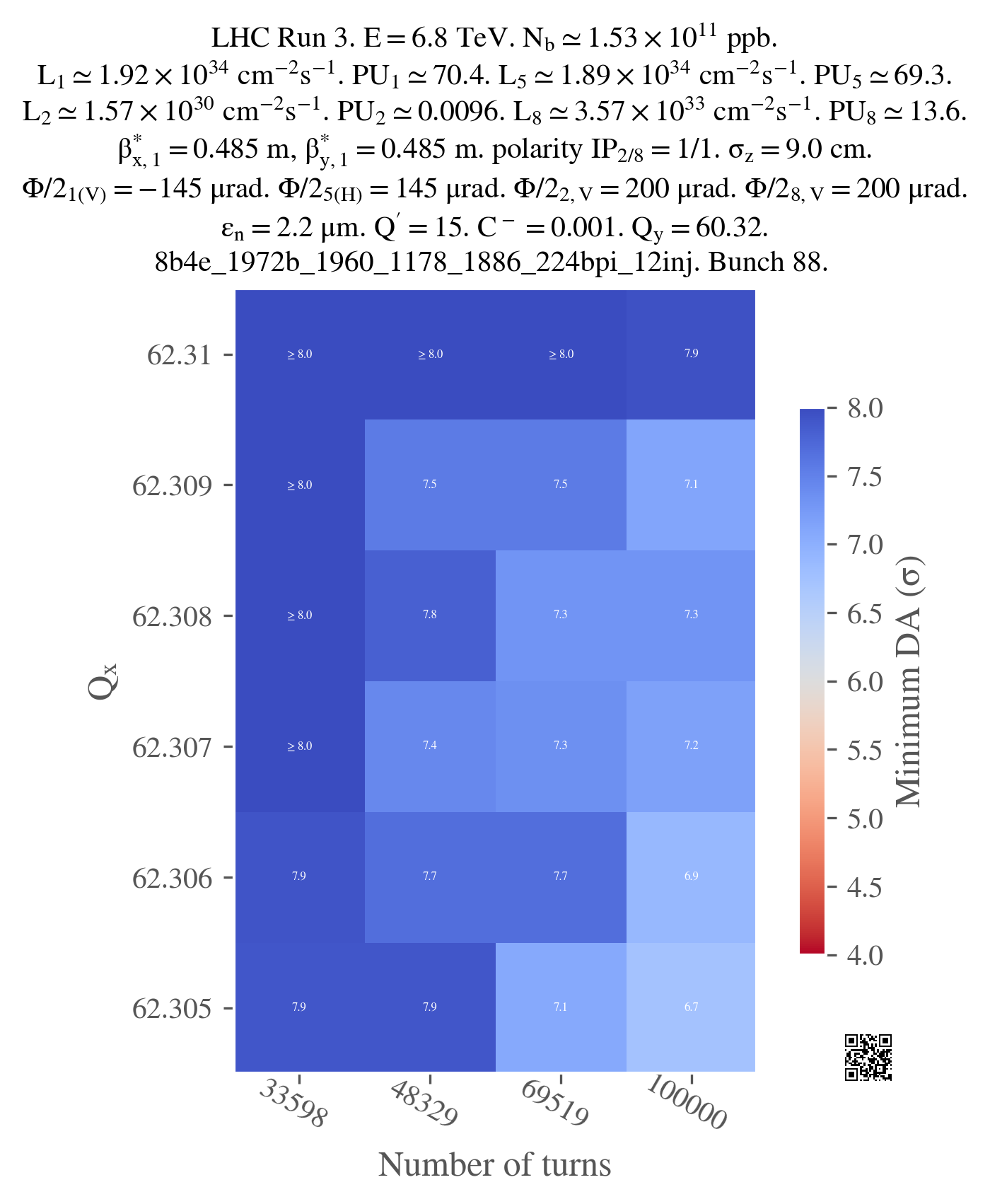
I used a png version as it's lighter to display for the browser but you should probably use a vectorized format for your plots, especially if you want to print them or include them in a presentation (you can always convert them to png afterwards if you need to).
Many examples of plotting are available in the case studies section, so you can check them out to see how to plot more realistic types of studies.