Doing an octupole scan along the tune superdiagonal
Octupole scans are an other type of scans that are frequently requested. Just like tune scan, they are usually done in second generation: the first one allows to convert the Mad sequence to a Xsuite collider (single job), while the second one enables to configure the collider and do the scan for various octupoles and tune values (tune values being on the superdiagonal). Let's give an example with the config_runIII.yaml configuration template.
You're getting better at this! I'm getting lazy...
You should have a reasonable understanding of the package by now. Therefore, details about the scripts and the configuration will not be explained in detail. If you need more information, please refer to the previous case studies.
Scan configuration
First, let's configure our scan. We want to do a two-dimensional scan, the first dimension being the tune on the superdiagonal (basically having qx and qy evolving together), and the second dimension being the octupole current.
# ==================================================================================================
# --- Structure of the study ---
# ==================================================================================================
name: example_oct_scan

# List all useful files that will be used by executable in generations below
# These files are placed at the root of the study
dependencies:
  main_configuration: config_runIII.yaml

structure:
  # First generation is always at the root of the study
  # such that config_runIII.yaml is accessible as ../config_runIII.yaml
  generation_1:
    executable: generation_1.py
    scans:
    common_parameters:
      # Needs to be redeclared as it's used for parallelization
      # And re-used ine the second generation
      n_split: 5

  # Second generation depends on the config from the first generation
  generation_2:
    executable: generation_2_level_by_nb.py
    scans:
      distribution_file:
        # Number of paths is set by n_split in the main config
        path_list: ["____.parquet", n_split]
      qx:
        subvariables: [lhcb1, lhcb2]
        linspace: [62.305, 62.330, 26]
      qy:
        subvariables: [lhcb1, lhcb2]
        expression: qx - 2 + 0.005
        concomitant: [qx]
      i_oct_b1:
        linspace: [-300, 300, 21]
      i_oct_b2:
        linspace: [-300, 300, 21]
        concomitant: [i_oct_b1]
As you can see, we use an expression to stipulate how qy should be generated from qx. In addition, we use the concomitant keyword to specify that qy should be scanned along with qx, i.e. not taking the cartesian product of the two variables. Similarly, for the octupole, we use the concomitant keyword to specify that the octupole current for beam 2 should be scanned along with the octupole current for beam 1. Note that, instead of a linspace for i_oct_b2, we could have used an expression to generate the octupole current from the octupole current for beam 1 (expression: i_oct_b1).
Study generation
We can now write the script to generate the study:
# ==================================================================================================
# --- Imports
# ==================================================================================================

# Import standard library modules
import os

# Import third-party modules
# Import user-defined modules
from study_da import create, submit
from study_da.utils import load_template_configuration_as_dic, write_dic_to_path

# ==================================================================================================
# --- Script to generate a study
# ==================================================================================================

# Load the template configuration
name_template_config = "config_runIII.yaml"
config, ryaml = load_template_configuration_as_dic(name_template_config)

# Do changes if needed
# config["config_simulation"]["n_turns"] = 1000000

# Drop the configuration locally
write_dic_to_path(config, "config_runIII.yaml", ryaml)

# Now generate the study in the local directory
path_tree, name_main_config = create(path_config_scan="config_scan.yaml", force_overwrite=False)

# Delete the configuration
os.remove("config_runIII.yaml")

# ==================================================================================================
# --- Script to submit the study
# ==================================================================================================

# In case gen_1 is submitted locally
dic_additional_commands_per_gen = {
    # To clean up the folder after the first generation if submitted locally
    1: "rm -rf final_* modules optics_repository optics_toolkit tools tracking_tools temp mad_collider.log __pycache__ twiss* errors fc* optics_orbit_at* \n"
    # To copy back the particles folder from the first generation if submitted to HTC
    # "cp -r particles $path_job/particles \n",
}

# Dependencies for the executable of each generation. Only needed if one uses HTC or Slurm.
dic_dependencies_per_gen = {
    1: ["acc-models-lhc"],
    2: ["path_collider_file_for_configuration_as_input", "path_distribution_folder_input"],
}

# Submit the study
submit(
    path_tree=path_tree,
    path_python_environment="/afs/cern.ch/work/u/user/private/study-DA/.venv",
    path_python_environment_container="/usr/local/DA_study/miniforge_docker",
    path_container_image="/cvmfs/unpacked.cern.ch/gitlab-registry.cern.ch/cdroin/da-study-docker:757f55da",
    dic_dependencies_per_gen=dic_dependencies_per_gen,
    name_config=name_main_config,
    dic_additional_commands_per_gen=dic_additional_commands_per_gen,
    one_generation_at_a_time=True,
)
As you can see, this script is very similar to the one from the previous case study.
One notable difference is that we don't modify the location of "acc-models-lhc" in the configuration since the path is already absolute.
In addition, note that we've specified one_generation_at_a_time=True. Therefore, even if you relaunch the script while some jobs of the second generation are ready to be launched (because the first generation is already partially finished), no jobs will be submitted. In this case, a generation can only be submitted all at once, i.e. if all the jobs from the generation above are finished (or failed). This is not so relevant for this example since there are only two generations, and generation has only 1 job, but it can be very useful for more complex studies (e.g. to run checks on all jobs of a generation, between generations submission).
Study post-processing and plotting
The script for post-processing and plotting is also very similar to the one from the previous case study:
# ==================================================================================================
# --- Imports
# ==================================================================================================
from study_da.plot import get_title_from_configuration, plot_heatmap
from study_da.postprocess import aggregate_output_data
# ==================================================================================================
# --- Postprocess the study
# ==================================================================================================
df_final = aggregate_output_data(
"example_oct_scan/tree.yaml",
l_group_by_parameters=["qx_b1", "qy_b1", "i_oct_b1", "i_oct_b2"],
generation_of_interest=2,
name_output="output_particles.parquet",
write_output=True,
only_keep_lost_particles=True,
force_overwrite=False,
)
# ==================================================================================================
# --- Plot
# ==================================================================================================
title = get_title_from_configuration(
df_final,
crossing_type="vh",
display_LHC_version=True,
display_energy=True,
display_bunch_index=True,
display_CC_crossing=False,
display_bunch_intensity=True,
display_beta=True,
display_crossing_IP_1=True,
display_crossing_IP_2=True,
display_crossing_IP_5=True,
display_crossing_IP_8=True,
display_bunch_length=True,
display_polarity_IP_2_8=True,
display_emittance=True,
display_chromaticity=True,
display_octupole_intensity=False,
display_coupling=True,
display_filling_scheme=True,
display_tune=False,
display_luminosity_1=True,
display_luminosity_2=True,
display_luminosity_5=True,
display_luminosity_8=True,
display_PU_1=True,
display_PU_2=True,
display_PU_5=True,
display_PU_8=True,
)
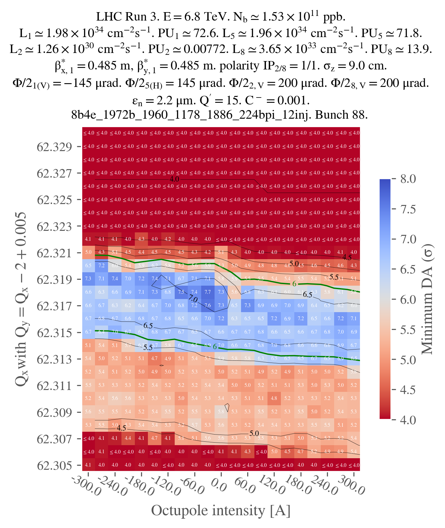
fig, ax = plot_heatmap(
df_final,
horizontal_variable="i_oct_b1",
vertical_variable="qx_b1",
color_variable="normalized amplitude in xy-plane",
plot_contours=True,
xlabel="Octupole intensity [A]",
ylabel=r"$Q_x$" + "with " + r"$Q_y = Q_x -2 + 0.005$",
title=title,
vmin=4.0,
vmax=8.0,
green_contour=6.0,
label_cbar="Minimum DA (" + r"$\sigma$" + ")",
output_path="oct_scan.png",
vectorize=False,
xaxis_ticks_on_top=False,
plot_diagonal_lines=False,
)
Note that, in this case, the parameters we used to group by the output data with are both the tune and the octupole current for beam 1 and beam 2. Also, in this case, we have to specify the type of crossing for the plotting since it can't be parsed from the configuration. Finally, a few adjustements are needed in the plot_heatmap function, they should be self-explanatory.
Just for illustration, here is the output of the plot (not vectorized):